Poles, Zeros, and Stability: The Z-Transform in Action

The $z$-transform is one of the most important mathematical tools in signal processing and system analysis. Through a series of fundamental questions, this post will guide you through its concepts, properties, and other applications.

Z-transform

Let’s begin with the first question. “What is the $z$-transform, and why do we need it?”. The $z$-transform is a mathematical tool for analyzing discrete-time signals and systems. It extends the Discrete-Time Fourier Transform (DTFT) by introducing a scaling factor $r$, which helps with stability and convergence. The $z$-transform is essential for LTI system analysis, stability checking, filter design, and difference equation solutions.

The $z$-transform of a discrete-time signal $x[n]$ is give by:

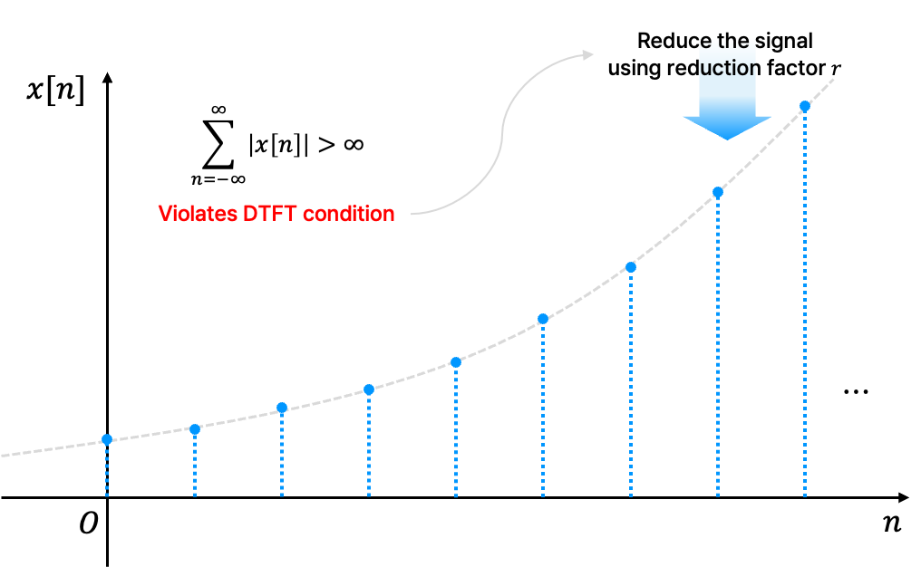
\[X(z)=\sum_{n=-\infty}^{\infty} x[n]z^{-n} \quad \text{where} \; z=re^{j\omega}\]

Why does the equation look like that? The term $e^{-j\omega n}$ is used in Fourier analysis to represent frequency components. The additional scaling factor $r^{-n}$ controls the growth/decay of signals and ensures convergence. So we can make an analysis even if the input signal is not making convergence.

---

Region of convergence

Then what value is to be set for $r$? The concept of Region of Convergence (ROC) emerges from this question. The ROC is the set of $z$-values where the Z-transform converges. It determines whether the system exists, and it plays a key role in stability analysis. For stability, the ROC must include the unit circle $\vert z \vert = 1$. We’ll see why below.

If we set $r = 1$, the $z$-transform reduces to the Discrete-Time Fourier Transform (DTFT).

\[X(\Omega)=\sum_{n = -\infty} ^{\infty} x[n]e^{-j\Omega n}\]

The key insight is that the Fourier transform analyzes frequency components, while the $z$-transform generalizes it by adding a scaling factor $r^{-n}$. If the ROC includes the unit circle, evaluating $X(z)$ at $z=e^{j\omega}$ gives the frequency response. Thus, the $z$-transform is a superset of the Fourier transform.

---

Poles and zeros

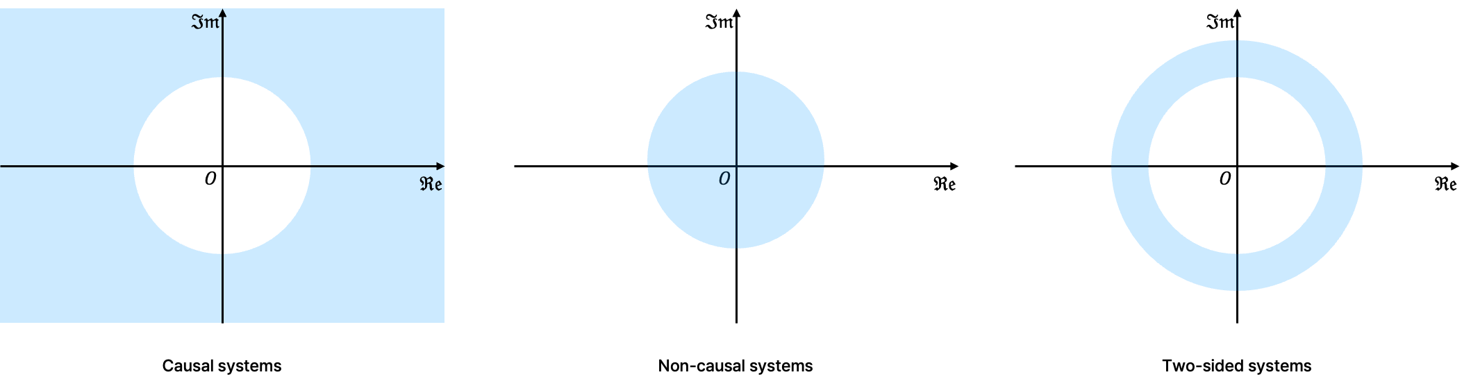
By the way, how do we check if a system is stable using the $z$-transform? We usually determine BIBO stability. BIBO means Bounded Input and Bouded Output. A discrete-time system is BIBO stable if the following equation satisfies:

\[\sum_{n=-\infty}^{\infty} |h[n]| < \infty.\]

To satisfy the equation above, the ROC must include the unit circle on $z$-plane. Also, we can determine the stability using the concept of ‘pole’. The poles of a system are the values of $z$ where $H(z)$ goes to infinity (denominator = 0). If all poles lie inside of unit circle, then we say system is stable on bounded input signal. Note that, we can only determine the system is stable or not.

The other concept that goes with ‘pole’ is ‘zeros’. Zeros are values of $z$ where $H(z)$ becomes zero (numerator = 0). Generally, poles are marked with ‘x’ in the $z$-plane and zeros are marked with ‘o’ in the $z$-plane. Poles determine stability, while zereos determine which frequencies are canceled.

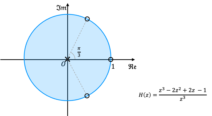Poles and zeros plotted on $z$-plane with sample response

At zero, the system completely cancels the corresponding frequency component. For example, if a system has a zero at z = $e^{j \pi / 4}$, it completely removes any signal component at $\omega = \pi / 4$. This is how notch filters work!

---

Convolution property of $z$-transfrom

Convolution in the time domain is multiplication in the $z$-domain, just like in Fourier analysis. This makes system analysis much easier.

\[x[n]*h[n]=X(\Omega) H(\Omega)=X(z)H(z)\]

---

Relationship between the $z$-transform and difference equation

As we’ve seen here a discrete-time linear time-invariant (LTI) system is often described using a difference equation, which relates the system’s output $y[n]$ to its input $x[n]$:

\[y[n]-\sum_{p=1}^{N}a_py[n-p] = \sum_{q=0}^{M} b_q x[n-q]\]

• $x[n]$: discrete-time input signal
• $y[n]$: output signal
• $a_k$: Feedback coefficients (related to system memory)
• $b_k$: Feedforward coefficients (how the input affects output)

This equation completely defines the system’s behavior and is fundamental in digital signal processing. The $z$-transform allows us to convert this time-domain equation into an algebraic equation in the $z$-domain, making it much easier to analyze.

\[Y(z)-a_1z^{-1}Y(z)-a_2z^{-2}Y(z)-\cdots -a_Nz^{-N}Y(z) \\ \quad = (b_0 + b_1z^{-1}+\cdots +b_Mz^{-M})X(z)\]

If we factor $Y(z)$ and rearrange the equation it will be:

\[H(z)=\frac{Y(z)}{X(z)} = \frac{b_0+b_1z^{-1}+\cdots+b_Mz^{-M}}{1-a_1z^{-1}-a_2z^{-2}-\cdots -a_Nz^{-N}}\]

Here, the denominator $X(z)$ comes form the left-hand side of the difference equation (the feedback part). Poles are the roots of $X(z)$, which define the system’s natural response (stability, transient behavior). On the other hand, the numerator $Y(z)$ comes from the right-hand side of the difference equation (the input reesponse). Zeros are the roots of $Y(z)$, which define how the system modifies the input.

So, whay I want to say here, the $z$-transform and the difference equation are deeply connected! The $z$-transform simplifies difference equations into an algebraic form, allowing us to easily analyze system behavior using poles and zeros.

---

Summary

The $z$-transform generalizes the Fourier Transform, making it a powerful tool for analysing discrete-time systems. It helps determine stability, system response, and frequency filtering with ease. Checking pole locations in the $z$-plane tells us everything about a system’s stability and behavior.