Table of Contents
Regularization is a method of preventing overfitting. It involves considering both the loss term and the weight parameters.
L1 Regularization
L1 regularization adds the L1 norm of the model parameters to the original loss term, such as MSE(Mean Squared Error) or RMSE (Root Mean Squared Error). When optimizing the model, we use the partial derivatives of the loss function. In this case, the total loss consists of two terms: the original loss and the regularization term.
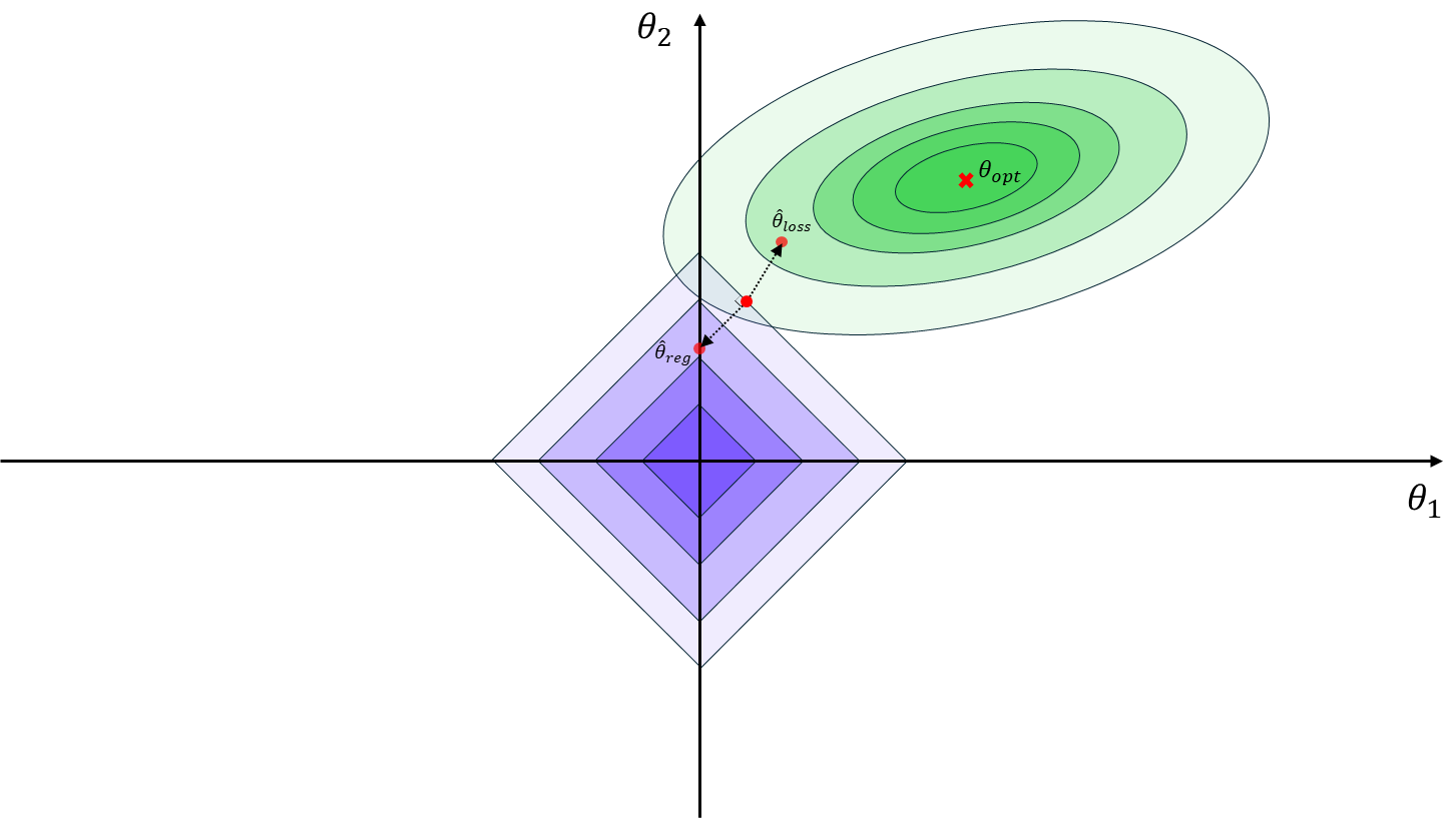
If we use the l1 norm as the regularization term, the derivative of the weight includes the sign of the weight (sign(w)). This causes the parameters to update by the same amount regardless of their magnitudes. As a result, some parameter values can become exactly zero, effectively performing feature selection. When a coefficient is zero, the corresponding feature does not influence the model. The equation for L1 regularization is as follows:
Taking the partial derivative to $W_i$ gives:
\[\frac{\partial\mathcal{L}}{\partial W_i} = \dots + \lambda\,\text{sign}({W_i})\]L2 Regularization
On the other hand, L2 regularization adds the L2 norm of the weight parameters, also known as the Frobenius norm, to the loss function to avoid overfitting. The Frobenius norm does not eliminate weight values but penalizes larger weights more heavily. This ensures that the weights are kept small but nonzero, distributing the penalty based on their magnitudes. Unlike L1 regularization, L2 regularization does not result in feature selection.
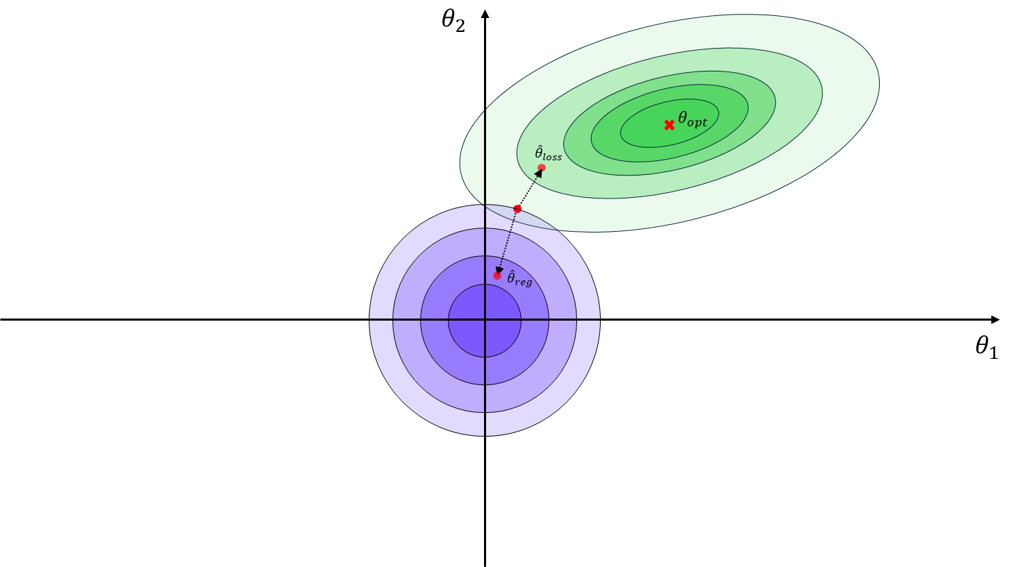
Meanwhile, L1 regularization is also known as Lasso regularization, and L2 regularization is called Ridge regularization. If we visualize the weight parameter values in a coordinate system, L1 regularization constrains the parameter contour into a diamond (or rhombus) shape, whereas L2 regularization creates circular contours. The gradient points in the direction of the steepest descent. In the case of L1 regularization, the diamond-shaped contours often lead to solutions where some parameters become zero, while the circular contours of L2 regularization direct the weights toward the center of the coordinate system but rarely to exact zeros.
Regularization and Maximum a Posteriori (MAP)
Regularization can also be interpreted in terms of Maximum a Posteriori (MAP) estimation. MAP incorporates prior distributions to maximize the posterior probability. L1 regularization assumes a Laplace prior distribution, whereas L2 regularization assumes a Gaussian prior distribution.
MAP (Maximum a Posteriori) estimation is defined by the following equation:
\[\hat{\theta}=\arg\max_\theta P(\theta \vert \mathcal{D})\]The equation represents the process of maximizing the probability of $\theta$ given the data $\mathcal{D}$. In this context, the parameter $\theta$ characterizes the data distribution. By applying Bayes’ theorem and taking them, we can rewrite the equation as:
\[\log P(\theta | \mathcal{D})=\log P(\mathcal{D}|\theta) + \log P(\theta) + \text{constants}\]Now, how is MAP estimation connected to the prior distribution used in regularization methods?
L1 Regularization and the Laplace Prior
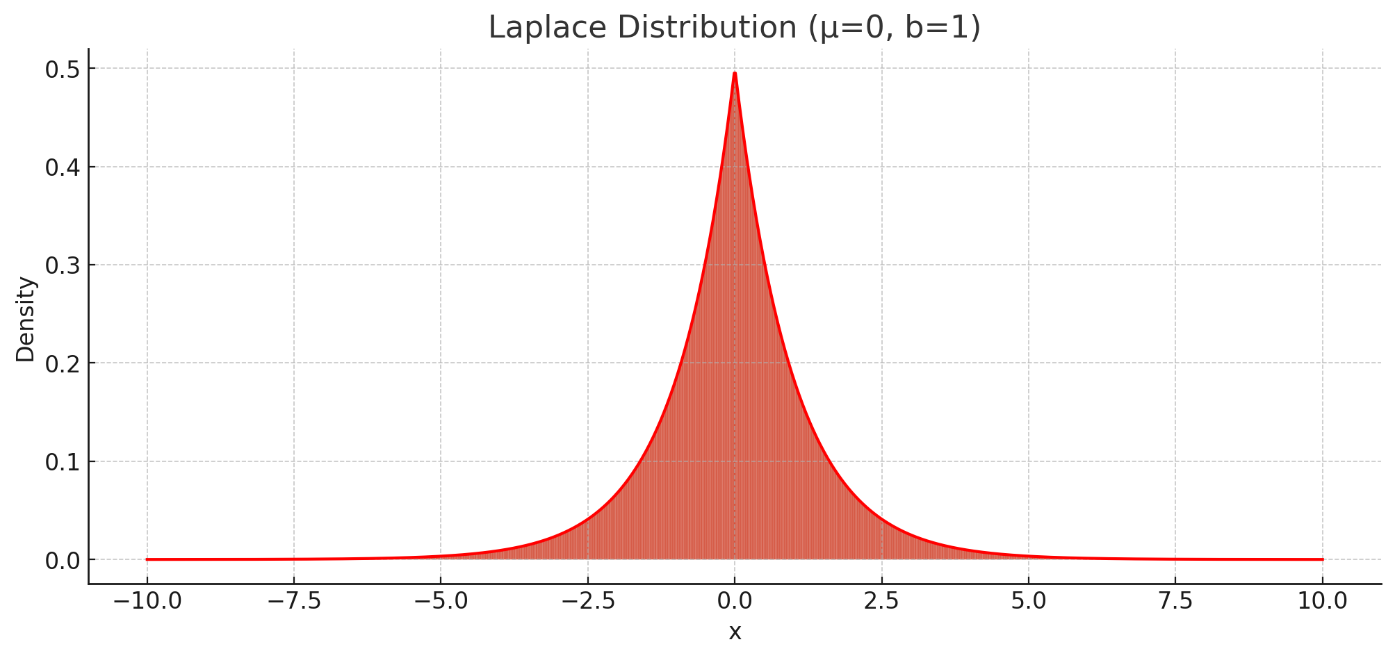 Laplace probability density function
First, the probability density function (PDF) of Laplace distribution is defined as:
\[P(W)=\prod_i \frac{\lambda}{2} \exp(-\lambda|W_i) \\ \log P(W)=\sum_i \log \frac{\lambda}{2}-\lambda |W_i|\]Using Maximum a Posteriori estimation, we include the prior term $\log P(W)$ in the loss function. Here, the term $-\lambda \vert W_i \vert$ matches the L1 regularization term. Thus, we can conclude that L1 regularization implicitly assumes a Laplace distribution as the prior for the weights.
L2 Regularization and the Gaussian Prior
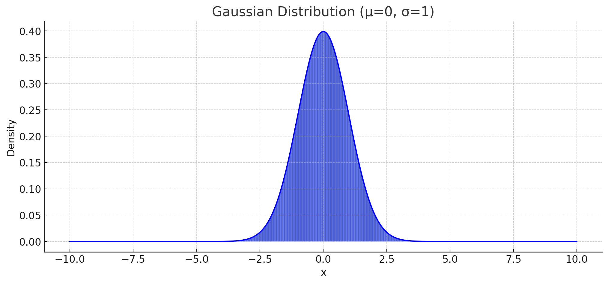 Gaussian probability density function
Now consider the PDF of the Gaussian distribution:
\[P(W)=\prod_i \frac{1}{\sqrt{2\pi \sigma^2}} \exp\left( -\frac{W_i^2}{2\sigma^2}\right) \\ \log P(W) = \sum_i -\frac{1}{2}\log(2\pi \sigma^2) - \frac{W_i^2}{2\sigma^2}\]In this case, the term $-\frac{W_i^2}{2\sigma^2}$ corresponds to the L2 regularization term. Therefore, we can conclude that L2 regularization assumes a Gaussian distribution as the prior for the weights.
Summary of Regularization and MAP
We’ve now seen how L1 and L2 regularization are and how they correspond to the prior distributions in MAP estimation: L1 regularization aligns with the Laplace distribution, while L2 regularization corresponds to the Gaussian distribution.
Regularization is an essential component of deep learning model implementation, helping to reduce overfitting and improve generalization. In practice, modern libraries like PyTorch make it straightforward to apply regularization. For instance, the weight_deacy parameter in PyTorch’s optimizers (e.g., torch.optim.SGD) implements L2 regularization. To use L1 regularization, you can manually add the L1 norm of the model parameters to the loss function.
if weight_decay != 0:
    # ...
    grad = grad.add(param, alpha=weight_decay)  # equivalent to: grad + alpha * param
And that’s it! With just a few lines of code, you can incorporate regularization into your deep-learning models.



Start the conversation